Example: chart all the data for the year 2012 in the grid

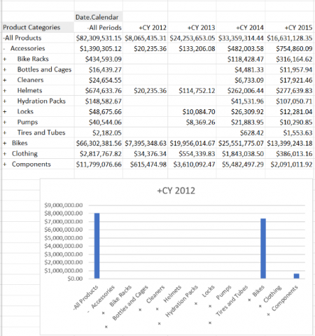
Below is an example of charting all the data shown for the calendar year 2012 in the grid

This example is based on the Adventure Works demo cube. 

1. Create a grid with the years across columns and Products on rows and then add three named ranges. Add named ranges in the Interaction tab in the Grid Properties window.
   • Named range 1
     • Name: CY2012Members
     • Scope: Workbook
     • Slice - Members, then add Date Calendar - CY 2012 to the slice
   • Named Range 2
     • Name: CY2012Data
     • Scope: Workbook
     • Slice - Data, then add Date Calendar - CY 2012 to the slice
   • Named range 3
     • Name: ProductMembers
     • Scope: Workbook
     • Members - Axis - Rows
       
       The lCY2012Members, CY2012Data, and ProductMembers list appears under the Named Ranges section.
2. Insert a new Excel column chart, right-click the column, and choose Select Data. The Select Data Source window appears.
3. Add a Legend Entry (Series) as Series name: =Sheet1!CY2012Members; Series values: =Sheet1!CY2012Data
4. Edit the Horizontal category labels to =Sheet1!ProductMembers and select OK. The chart appears:

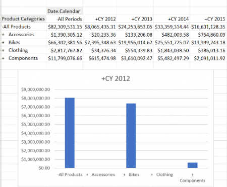
The chart updates its members and data when the grid changes: