

Standard Anaplan XL formatting and cell protection originate from the AnaplanXLFormats worksheet. You can define additional ranges of cells to control formatting and locking. These ranges use the same rules as the format sheet (dimension, member, or data cell) but don’t include spacer cells between cells.
Anaplan XL process cell formatting and protection rules in sequence:
- Base Grid formatting: Anaplan XL evaluates default hierarchy formatting, member styles, and locked status rules defined on the AnaplanXLFormats worksheet.
- Custom formatting areas (driver ranges): Anaplan XL overlays formatting and cell locking from any user-defined range configured under the Custom formatting areas section for Range in the Appearance tab of the Grid Properties window.
The grid applies these additional rules after the format sheet’s rules. The grid tracks changes to these independently of its refresh status. You can dynamically drive cell formatting and locking from Excel formulas or an external data source, such as a SQL query.
You can add custom formatting and locking areas under the Custom formatting areas section. In the Appearance tab of the Grid Properties window, select the + icon for Range and select the range in your workbook to determine the formatting and locking.
Build the dynamic driver grid
You can build a report to automatically unlock future forecast periods while locking historical actuals and apply cell formatting.
- Create a grid report.
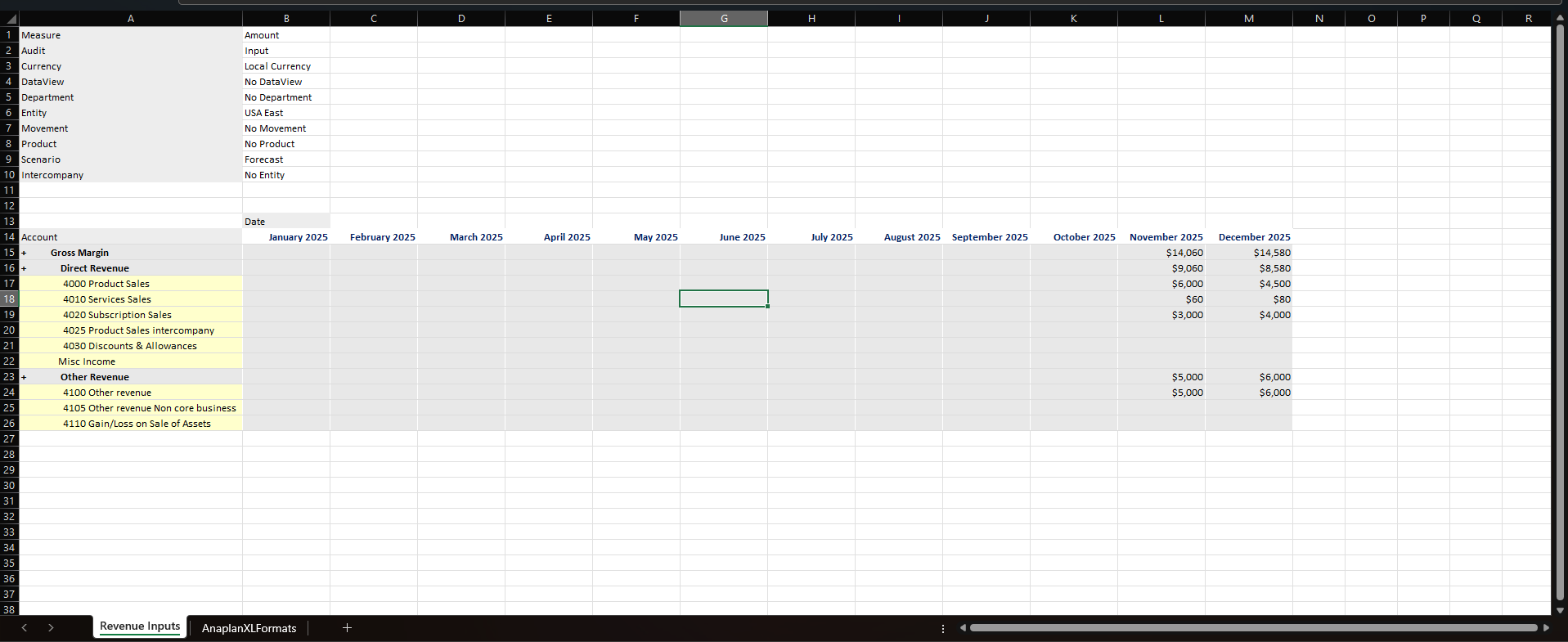
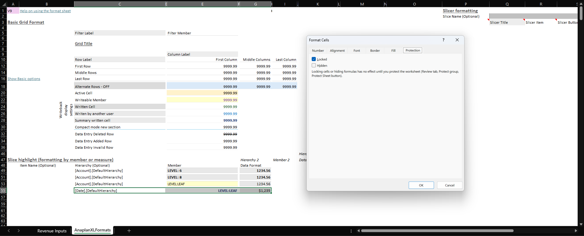
- Apply formatting and lock dimensions, members, or data cells in the report using the AnaplanXLFormats sheet.
- Select a dimension, member, or data cell (for example, Date), right-click, and select Format Cells... > Protection > Locked.
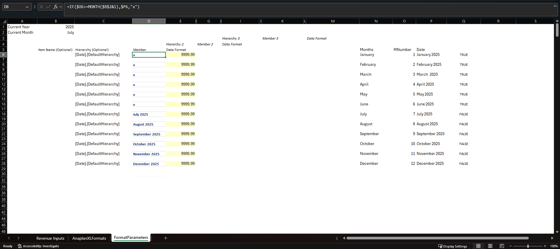
- Create a new worksheet or copy the AnaplanXLFormats worksheet to store the formatting and locking parameters.
Name the new worksheet, for example, FormatParameters. You can hide the new worksheet and AnaplanXLFormats from users before publishing.
Note: If you copy the AnplanXLFormats worksheet, you will only need the items below row 36. Copying the sheet keeps the column names consistent, making it easier to reference the cells you format or lock. If you copied the AnaplanXLFormats worksheet, you need to delete the extra columns between Hierarchy (Optional), Member, and Hierarchy 2.
- Create a reference date cell. For example, put the current year in cell
B1and the current month inB2. - Name the columns the same names as the columns in the Slice highlight (formatting by member or measure) section of the AnaplanXLFormats worksheet. This is optional.
- Under the Hierarchy (Optional) column, type the same dimension and hierarchy being used in the AnaplanXLFormats worksheet, such as
[Date].[DefaultHierarchy]in all the appropriate rows. - Add columns before the Item Name (Optional) column or after the last Data Format:
For example:- A Months column contains January through December.
- The MNumber column contains the Excel formula
= MONTH ($N6 & 1)to return the month number. - The Date column contains an Excel formula
=CONCATENATE($N6 & " " & $B$1)to return the month and the current year.
- In the first Member column, enter a formula to determine whether the member is open for the Forecast scenario, such as
=IF($O6>=MONTH($B$2&1),$P6,"x"), then unlock the cells. - In the first Data Format column, type a number or text, apply Excel formatting, and unlock the cells.
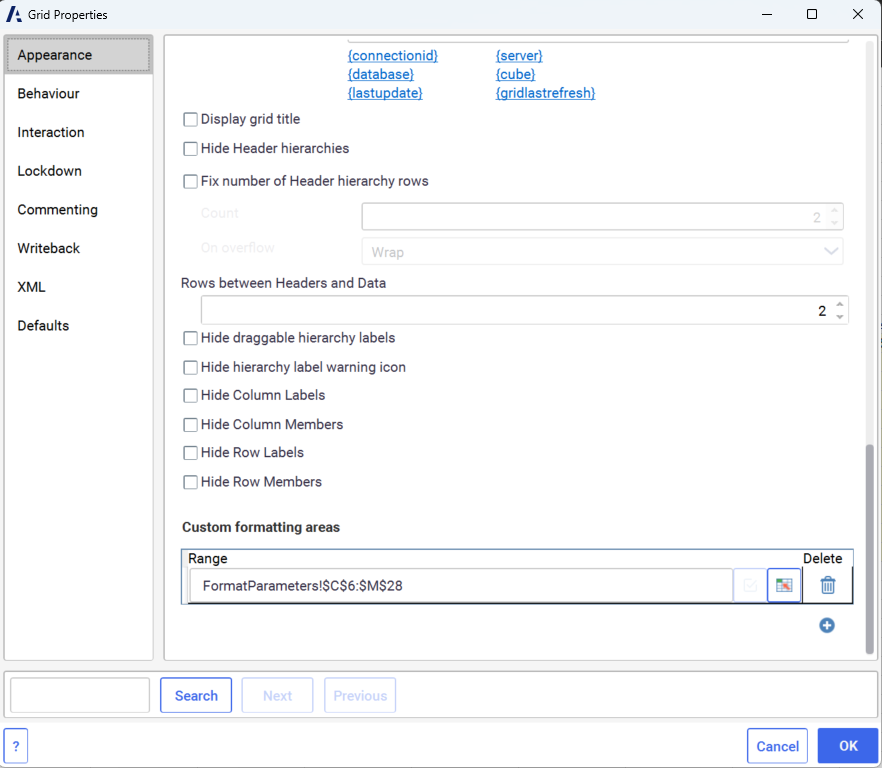
10. Select the worksheet with the grid report, right-click in the grid, and choose Anaplan XL > Properties... > Appearance tab.
11. Under the Custom formatting areas section, select the + icon.
12. Select the range on the worksheet tab containing the formatting and locking parameters, such as FormatParameters!$C$6:$M$28.
13. Go to the worksheet with the grid report and select Grid > Refresh.

